[RNH post #9] Progress Report (24th of July)

Progress is going as planed in my mid-term summary :). 

A short summary of what was done on the last weeks is described in the points below:

• The functions to fit the diffusion kurtosis tensor are already merged to the main Dipy's repository (you can see the merged work here).
• The functions to extract kurtosis statistics were submitted in a separate pull request. Great advances on the validation of these functions were done according to the next steps pointed in the mid-term summary. Particularly, I completed the comparisons between the analytical solutions with simpler numerical methods (for nice figures of these comparisons, see below the subsection "Advances on the implementation of DKI statistics").
• At the same time that I was waiting for the revision of the work done on kurtosis tensor fitting and statistic estimation, I started working on functions to estimate the direction of brain white matter fibers from diffusion kurtosis imaging. This work is happening in a new created pull request. For the mathematical framework of this implementation and some nice figures of the work done so far, you can see below the subsection "DKI based fiber estimates".

Advances on the implementation of DKI statistics

Improving the speed performance of functions - As mentioned on the last points of my mid-term summary, some features on the functions for estimating kurtosis statistics to reduce the processing time were added. At the time of the mid-term evaluation, I was planing to add some optional inputs to receive a mask pointing the relevant voxels to process. However, during the last weeks, I decided that a cleaver way to avoid processing unnecessary background voxels was to create a subfunction that automatically detects these voxels (detecting where all diffusion tensor elements are zero) and exclude them. In addition, I also vectorized parts of the codes (for details on this, see directly the discussion on the relevant pull request page). Currently, reprocessing the kurtosis measures shown in Figure 1 of my post #6 is taking around:

• Mean Kurtosis - 14 mins
• Radial Kurtosis - 7 mins
• Axial Kurtosis - 1 min

Using ipython profiling techniques, I also detected the parts of the codes that are more computationally demanding. Currently, I have been discussing with members of my mentoring organization the possibility of converting this function in cython.

Comparison between mean kurtosis analytical and approximated solutions. Mean Kurtosis (MK) corresponds to the average of the kurtosis values along all spatial directions. Therefore, an easy way to estimate MK is to sample directional kurtosis values in evenly sampled directions and compute their average. This procedure can be very easy to implement, however it has some pitfalls as requiring a sufficient number of direction samples and being dependent on the performance of the direction sampling algorithms. Fortunately, this pitfalls can be overcome using an analytical solution that was proposed by Tabesh and colleagues.

In previous steps of my GSoC project, I had already implemented the MK estimation functions according to the analytical solution. However, I decided to implement also the directional average since it could be useful to evaluate the analytical approach. In the figure below, I run this numerical estimate for different number of directions, to analyse how many directions are required so that the directional kurtosis average approaches the analytical mean kurtosis solution.

Figure 1 - Comparison between the MK analytical (blue) and numerical solutions (red). The numerical solution is computed relative to a different number of direction samples (x-axis). 

From the figure above, we can see that the numerical approach never reaches a stable solution. Particularly, large deviations are still observed even when a large number of directions is sampled. After a careful analysis, I noticed that this was caused by imperfections on the sphere dispersion algorithm strategies to sample evenly distributed directions.

Due to the poor performance, I decided to completely remove the MK numerical solution from the DKI implementation modules. This solution is only used on the code testing procedures.  


Comparison between radial kurtosis analytical and approximated solutions. Radial kurtosis corresponds to the average of the kurtosis values along the perpendicular directions of the principal axis, i.e. the direction of non-crossing fibers. Tabesh and colleagues also proposed an analytical solution for this kurtosis statistic. I implemented this solution in Dipy on my previous steps of the GSoC project. Nevertheless, based on the algorithm described in my post #8, radial kurtosis can be estimated as the average of exactly evenly perpendicular direction samples. The figure below shows the comparison between the analytical solution and the approximated solution for a different number of perpendicular direction samples.

Figure 2 - Comparison between the RK analytical (blue) and numerical solutions (green). The numerical solution is computed relative to a different number of direction samples (x-axis).

Since, opposite to the MK case, the algorithm to sample perpendicular directions does not depend on sphere dispersion algorithm strategies, the numerical method for the RK equals the exact analytical solution after a small number of sample directions.

Future directions of the DKI statistic implementation. Having finalized the validation of the DKI statistic implementation, the last step of the DKI standard statistic implementation is to replace the data used on the sample usage script by an HCP-like dataset. As mentioned on my post #7, the reconstructions of the dataset currently used on this example seems to be corrupted by artifacts. After discussing with an expert of the NeuroImage mailing list, these artefacts seem to be caused by an insufficient SNR for fitting the diffusion kurtosis model.

DKI based fiber direction estimates

Mathematical framework. This fiber direction estimation is done based on the orientation distribution function as proposed by Jensen and colleagues (2014). The orientation distribution function (ODF) gives the probability that a fiber is aligned to a given direction and it can be estimated from the diffusion and kurtosis tensors using the following formula:

where α is the radial weighting power, Uij is the element ij of the dimensionless tensor U which is defined as the mean diffusivity times the inverse of the diffusion tensor (U = MD x iDT), Vij is defined as

and ODFg the Gaussian ODF contribution which is given by: 

Implementation in python 1. In python, this expression can be easily implemented using the following command lines:

(Note to a description of what from_lower_triangular does, see Dipy's DTI module). 


Results. in the figure below, I show a ODF example obtained from the simulation of two white matter crossing fibers. 

Figure 3 - DKI -ODF obtained from two simulated crossing fibers. Maxima of the ODF correspond to the direction of the crossing fibers.

From the figure above, we can see that the ODF has two directions with maxima amplitudes which correspond to the directions where fibers are aligned.


Implementation in python 2. The lines of codes previously presented correspond to a feasible implementation of Jensen and colleagues formula. However, for the implementation of the DKI-ODF in dipy, I decided to expand the four for loops and use kurtosis tensor symmetry to simplify this expansion. The resulting code is as follow:

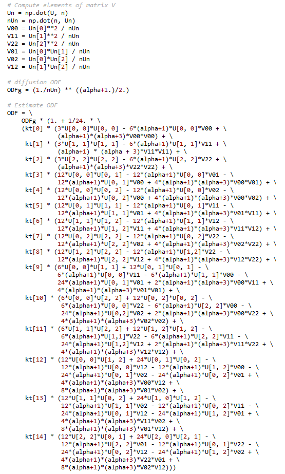
This implementation of the ODF can look less optimized, but in fact it involves a smaller number of operations relative to the four for loops of the algorithm in "Implementation in python 1". Particularly, this version of the code is more than 3 times faster!

Future directions of the DKI-ODF implementation. An algorithm to find the maxima of the DKI-ODF will be implemented. The direction of maxima ODF will be used as the estimates of fiber direction that will be useful to obtain DKI based tractography maps (for a reminder of what is a tractography map, see my post #3).

[RNH post #8] Perpendicular directions samples relative to a given vector

As I mentioned in the mid-term summary, one of my next steps is to implement some numerical methods to compute the standard kurtosis measures to evaluate their analytical solution. 

The numerical method for the perpendicular kurtosis requires samples of perpendicular directions to a given vector v.  

I am posting here the mathematical basis of this function which will be implemented in module dipy.core.geometry and named as perpendicular_directions.

Function's Algorithm

Inputs: 

• Vector v: Perpendicular directions are sampled relative to this vector.
• N: Number of perpendicular directions

Step 1) The N directions are first sampled in the unit circumference parallel to the y-z plane (plane normal to the x-axis), as shown the figure below.

Fig 1. First step of perpendicular_directions algorithm.

Coordinates of the perpendicular directions are therefore initialized as:

           (Eq.1)

where ai are the angles sampled for [0, 2*pi [. To perform N samples, the angle between two adjacent directions is given by 2*pi / N.

  

Step 2) Sampled directions are then rotated and aligned to the plane normal to vector v (see figure below).

Fig 2. Second step of perpendicular_directions algorithm.

Mathematically, this is done by multiplying each perpendicular directions ni by a rotational matrix. The final perpendicular directions di are given by:

    (Eq.2)

The rotational matrix in Eq.2 is constructed as the reference of frame basis in which the first basis axis is the vector v, while the other two basis axis are any pair of orthogonal directions pair relative to vector v. These orthogonal vectors are named here as vector e and vector k. For the implementation of function perpendicular_directions, vectors e and k are estimated using the following procedure:

    1) The direction of e is defined as the normalized vector defined by the cross product between vector v and the unit vector aligned to x-axis, i.e [1, 0, 0]. After normalizing, the final coordinates of e are:

 (Eq.3)

    2) k is directly defined as the cross product between vectors v and e. The coordinates of this vector are:

 (Eq. 4)

From equations 2, 3 and 4, the coordinates of the perpendicular directions relative to vector v are give as:

(Eq. 5)

Note that Eq. 5 has a singularity when vector v is aligned to the x-axis. To resolve this singularity, perpendicular directions are first defined in the x-y plane and vector e is computed as the normalized vector given by the cross product between vector v and the unit vector aligned to the y-axis, i.e [0, 1, 0]. Following this, the coordinates of the perpendicular directions are given as:

 (Eq. 6)

[RNH Post #7] Artifacts in Dipy's sample data Sherbrooke's 3 shells

Hi all,

Just to report an issue that I am currently trying to figure out!

As I showed on my previous post my first diffusion kurtosis reconstructions are looking very good. However when I try to process the Dipy's multi-shell dataset sample Sherbrooke 3 shells, kurtosis measures seem to be widely corrupted by implausible high negative values see figure below:

Fig.1 - Diffusion kurtosis standard measures obtain from the Sherbrooke 3 shells Dipy's sample dataset.

[RNH Post #6] Mid-Term Summary

We are now at the middle of the GSoC 2015 coding period, so it is time to summarize the progress done so far and update the plan for the work of the second half part of the program.

Progress summary

Overall a lot was achieved! As planed on my project proposal, during the first half of the coding period, I finalized the implementation of the first version of the diffusion kurtosis imaging (DKI) reconstruction module. Moreover, some exciting extra steps were done! 

Accomplishing the first steps of the project proposal

1) The first accomplished achievement was merging the work done on the community bonding period to the main master Dipy repository. This work consisted on some DKI simulation modules that can be used to study the expected ground truth kurtosis values of white matter brain fibers. In this project, these simulations were useful to test the real brain DKI processing module. The documentation of this work can be already found in Dipy's website. 

2) The second achievement was finalizing the procedures to fit the DKI model on real brain data. This was done from inheritance of a module class already implemented in Dipy, which contains the implementation of the simpler diffusion tensor model (for more details on this you can see my previous post). Completion of the DKI fitting procedure was followed by implementation of functions to compute the ordinary linear least square fit solution of the DKI model. By establishing the inheritance between the DKI and diffusion tensor modules, duplication of code was avoided and the standard diffusion tensor measures were automatically incorporated. The figure below shows an example of these standard measures obtained from the new DKI module after the implementation of the relevant fitting functions.

Figure 1 - Real brain standard diffusion tensor measures obtained from the DKI module, which included the diffusion fractional anisotropy (FA), the mean diffusivity (MK), the axial diffusivity (AD) and the radial diffusivity (RD). The raw brain dataset used for the images reconstruction was kindly provided by Maurizio Marrale (University of Palermo).

3) Finally, from the DKI developed fitting functions, standard measures of kurtosis were implemented. These were based on the analytical solutions proposed by Tabesh and colleagues which required, for instance, the implementation of sub-functions to rotate 4D matrices and to compute Carlson's incomplete elliptical integrals.  Having implemented the analytical solution of standard kurtosis measure functions, I accomplished all the work proposed for the first half of the GSoC. Below I am showing the first real brain images reconstructed kurtosis from the new implemented modules. 

Figure 2 - Real brain standard kurtosis tensor measures obtained from the DKI module, which included the mean kurtosis (MK), the axial kurtosis (AK), and radial kurtosis (RK). The raw brain dataset used for the images reconstruction was kindly provided by Maurizio Marrale (University of Palermo).


Extra steps accomplished

Some extra steps were also accomplished during the first half of the GSoC program. In particular, from the feedback that I obtained at the International Society for Magnetic Resonance in Medicine (ISMRM) conference (see my fourth post), I decided to implement an additional DKI fitting solution - the weighted linear least square DKI fit solution. This fit is considered to be one of the most robust fitting approaches in recent DKI literature (for more details see my previous post). Therefore, having this method implemented, I am insuring that the new Dipy's DKI modules are implemented according to the most advanced DKI state of art.

To show how productive was the ISMRM conference for the project, I am sharing you a photo that I took at the conference with one of the head developers of Dipy - Eleftherios Garyfallidis.

Figure 3 - Photo taken at the ISMRM conference - I am wearing the Dipy's T-shirt at the right side of the photo and in the left side you can see the head Dipy's developer Eleftherios Garyfallidis.

Next steps

After discussing with my mentor, we agreed that we should dedicate more time on the first part of the project proposal, i.e. improving the DKI reconstruction module. Due to the huge extent of code and the math complexity of this module, I will dedicate a couple of weeks more in improving the module's performance, quality of code testing and documentation. In this way, we decided to postpone the two last milestones initially planed for the second half term of the GSoC to the last three weeks of the GSoC coding period. 

The next steps of the updated project plan are as described in the following points: 

1) Merge the pull requests that contain the new DKI modules with the master's Dipy repository. To facilitate the revision of the implemented functions by the mentoring organization, I will split my initial pull request into smaller pull requests.

2) At the same time that the previous developed code is reviewed, I will implement new features on the functions for estimating kurtosis parameters to reduce processing time. For instance, I will implement some optional variables that allow each method to receive a Boolean mask to point the image voxels to be processed. This will save the time wasted on processing unnecessary voxels as from the background.

3) I will also implement simpler numerical methods for a faster estimation of the standard DKI measures. These numerical methods are expected to be less accurate that the analytical solutions already implemented, however they provide alternatives less computationally demanding. Moreover, they will provide a simpler mathematical framework which will be used to further validate the analytical solutions.

4) Further improvements of the weighed linear least square solution will be performed. In particular, the weights' estimations used on the fit will be improved by an iterative algorithm as described on recent DKI literature. 

5) Finally, the procedures to estimate from DKI concrete biophysical measures and white matter fiber directions will be implemented as I described on the initial project proposal.